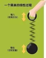
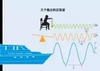
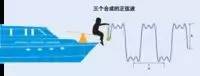
The time domain is a description of the relationship of a mathematical function or physical signal to time. For example, a time domain waveform of a signal can express a change in signal over time. If discrete time, function or signal in the time domain is considered, the values ​​at each discrete time point are known. If continuous time is considered, the value of the function or signal at any time is known. When studying the signal in the time domain, the oscilloscope is often used to convert the signal to its time domain waveform. The frequency domain frequency domain is a coordinate system used to describe the characteristics of a signal in terms of frequency. The description of any thing needs to be carried out in many aspects, and the description of each aspect is only a part of the information we provide to know this thing. For example, there is a car in front of me, I can describe it in terms of color: length, height. Aspect 2: Displacement, brand, price. For a signal, it also has many aspects of its characteristics. Such as the variation of signal strength with time (time domain characteristics), which signals are synthesized by which single frequency signals (frequency domain characteristics) Time domain time domain is the range of basic variables in time when analyzing research problems. The time domain is a description of the relationship of a mathematical function or physical signal to time. For example, a time domain waveform of a signal can express a change in signal over time. If discrete time, function or signal in the time domain is considered, the values ​​at each discrete time point are known. If continuous time is considered, the value of the function or signal at any time is known. When studying the signal in the time domain, the oscilloscope is often used to convert the signal to its time domain waveform. The time domain is the real world and the only domain that actually exists. Because our experiences are developed and validated in the time domain, we have become accustomed to events happening in chronological order. When evaluating the performance of a digital product, it is usually analyzed in the time domain because the performance of the product is ultimately measured in the time domain. The clock waveform shown in Figure 2.1 below. Clock waveform Figure 2.1 Typical Clock Waveform As you can see from the figure above, the two important parameters of the clock waveform are the clock cycle and rise time. The figure shows the clock period of the 1 GHz clock signal and the 10-90 rise time. The fall time is generally shorter than the rise time, and sometimes more noise occurs. The clock cycle is the time interval in which the clock cycle repeats, usually measured in ns. The clock frequency Fclock, that is, the number of clock cycles in one second, is the reciprocal of the clock cycle Tclock. The Fclock=1/Tclock rise time is related to the time it takes for the signal to transition from low to high. There are usually two definitions. One is the 10-90 rise time, which is the time it takes for the signal to transition from 10% of the final value to 90%. This is usually a default expression that can be read directly from the time domain map of the waveform. The second definition is 20-80 rise time, which is the time elapsed from 20% of the final value to 80%. The fall time of the time domain waveform also has a corresponding value. According to the logic series, the fall time is usually shorter than the rise time, which is caused by the design of a typical CMOS output driver. In a typical output driver, the p-tube and the n-tube are connected in series between the power rails Vcc and Vss, and the output is connected in the middle of the two tubes. At any one time, only one transistor is turned on, and which tube is conducting depends on the high or low state of the output. The frequency domain frequency domain uses frequency as a basic variable when analyzing problems. The frequency domain frequencydomain is a coordinate system used to describe the frequency characteristics of a signal. The description of any thing needs to be carried out in many aspects, and the description of each aspect is only a part of the information we provide to know this thing. For example, there is a car in front of me, I can describe it in terms of color: length, height. Aspect 2: Displacement, brand, price. For a signal, it also has many aspects of its characteristics. Such as the variation of signal strength with time (time domain characteristics), which signals are synthesized by which single frequency signals (frequency domain characteristics) Frequency domain analysis Frequency domain (frequency domain) - The independent variable is the frequency, that is, the horizontal axis is the frequency, and the vertical axis is the amplitude of the frequency signal, which is usually the spectrum. The spectrogram depicts the relationship between the frequency structure and frequency of the signal and the amplitude of the signal. When performing time domain analysis on a signal, sometimes the time domain parameters of some signals are the same, but it does not mean that the signals are identical. Because the signal changes not only with time, but also with information such as frequency and phase, it is necessary to further analyze the frequency structure of the signal and describe the signal in the frequency domain. The transformation of the dynamic signal from the time domain to the frequency domain is mainly achieved by Fourier series and Fourier transform. The periodic signal is dependent on the Fourier series, and the aperiodic signal is transformed by Fourier transform. Example A simple example of frequency domain analysis can be illustrated by Figure 1: A child's toy in a simple linear process. The linear system includes a weight that is suspended by a spring mounted by a handle. The child controls the position of the weight by moving the handle up and down. Anyone who has played this game knows that if the handle is moved more or less in a sine wave, the weight will start to oscillate at the same frequency, even though the weight is oscillating with the handle. The move is not synchronized. Only when the spring is not fully extended, the weight and spring will move synchronously and operate at a relatively low frequency. As the frequency gets higher and higher, the phase of the weight oscillation may be more advanced than the phase of the handle, and may be more lagging. At the natural frequency point of the process object, the height of the weight oscillation will reach the highest. The natural frequency of the process object is determined by the mass of the weight and the strength factor of the spring. When the input frequency is more and more larger than the natural frequency of the process object, the amplitude of the weight oscillation will tend to decrease, and the phase will be more lagging (in other words, the amplitude of the weight oscillation will be less and less, and the phase lag will become more and more Big). In the case of extremely high frequencies, the weight moves only slightly, as opposed to the direction of movement of the handle. All linear process objects of the Bode diagram exhibit similar characteristics. These process objects convert the input of the sine wave into the output of a sine wave of the same frequency, except that the amplitude and phase of the output and input change. The amount of change in amplitude and phase depends on the phase lag and gain of the process object. The gain can be defined as “the proportional coefficient between the amplitude of the output sine wave and the amplitude of the input sine wave after amplification by the process objectâ€, and the phase lag can be defined as “the degree to which the output sine wave is compared with the input sine wave and the output signal lags†. Unlike the steady state gain K value, the "gain and phase lag of the process object" will vary depending on the frequency of the input sine wave signal. In the above example, the spring-heavy object does not significantly change the amplitude of the low frequency sine wave input signal. This means that the object has only one low frequency gain factor. When the signal frequency is close to the natural frequency of the process object, since the amplitude of the output signal is greater than the amplitude of the input signal, the gain coefficient is greater than the coefficient at the low frequency. When the toy in the above example is swiftly shaken, the high frequency gain of the process object can be considered to be zero because the weight is hardly oscillated. The phase lag of the process object is an exceptional factor. Since the weight oscillates synchronously with the handle when the handle moves very slowly, in the above example, the phase lag begins with a low frequency input signal close to zero. At high frequency input signals, the phase lag is "-180 degrees", that is, the weight moves in the opposite direction to the handle (so we often use 'lag 180 degrees' to describe the reverse motion of the two). . The Bode map shows the complete spectrum of the system gain and phase lag in the frequency range of 0.01-100 radians per second for spring-heavy objects. This is an example of a Bode map, a graphical analysis tool invented by Hendrick Bode of Bell Labs in the 1940s. The tool can be used to determine the vibration amplitude and phase of the corresponding output signal when the process object is driven by a sine wave input signal of a specific frequency. To obtain the amplitude of the output signal, it is only necessary to multiply the amplitude of the input signal by the "gain factor corresponding to the frequency in the Bode diagram". To obtain the phase of the output signal, it is only necessary to add the phase of the input signal to the "phase lag value corresponding to the frequency in the Bode diagram". The gain coefficient and phase lag value of Fourier's theorem in the Bode diagram of the process object reflect the very certain characteristics of the system. For a well-controlled control engineer, the map needs to know the relevant process object. All the features are told to him accurately. Thus, the control engineer can use this tool to not only predict the "system response of the system's future control of the sine wave", but also the "system response to any control action". The Fourier theorem makes the above analysis possible, which shows that any successively measured timing or signal can be represented as an infinite superposition of sinusoidal signals of different frequencies. The mathematician, Fu Liye, proved this famous theorem in 1822 and created a well-known algorithm called Fourier Transform, which uses the directly measured raw signal to calculate the different sine wave signals in an additive manner. Frequency, amplitude and phase. In theory, Fourier transforms and Bode plots can be used in combination to predict the response that occurs when a linear process object is affected by the timing of the control action. See below for details: 1) Using the mathematical method of Fourier transform, the control effect provided to the process object is theoretically decomposed into the signal composition or spectrum of different sine waves. 2) Using the Bode plot, it can be determined that each sine wave signal changes as it passes through the object. In other words, the change in amplitude and phase of the sine wave at each frequency can be found on the graph. 3) Conversely, by using the inverse Fourier transform method, each individually changed sine wave signal can be converted into a signal. Since the inverse Fourier transform is essentially an additive process, the linear characteristics of the process object will ensure that the set of individual effects produced by the "various theoretical sine waves calculated in the first step" should be equivalent. The effect produced by the "accumulated set of different sine waves". Therefore, the total signal calculated in the third step will represent the "actual value of the process object when the provided control action is input to the process object". Note that none of the above steps consists of a single sine wave generated by the controller drawn on the graph. All of these frequency domain analysis techniques are conceptual. This is a convenient mathematical method that uses a Fourier transform (or a closely related Laplace transform) to convert a time domain signal into a frequency domain signal, and then use a Bode diagram or some other frequency domain analysis tool to solve the problem at hand. Some problems, finally using the inverse Fourier transform to convert the frequency domain signal into a time domain signal. The vast majority of control design problems that can be solved with this method can also be solved by direct manipulation in the time domain, but for calculations, the method of using the frequency domain is usually simpler. In the above example, multiplication and subtraction are used to calculate the spectrum of the actual value of the process, and the actual value of the process is obtained by Fourier transforming the given control action, and then comparing with the Bode diagram. Three sine waves Correct accumulation of all sinusoids produces a signal of the type that is predicted by the Fourier transform. When this phenomenon is sometimes not intuitive, an example might help to understand. Think again about the child's weights in the above example - the spring toy, the seesaw on the playground, and the boat on the outer ocean. Imagine that the ship rises and falls on the sea in the form of a sine wave of frequency w and amplitude A. We also assume that the seesaw is also oscillating in the form of a sine wave with a frequency of 3w and an amplitude of A/3, and the child is at a frequency. Shake the toy in the form of a sine wave of 5w and amplitude A/5. 'Three separate sine wave waveforms' have shown that if we observe three different sinusoidal motions separately, each sine wave motion will take its form. Now suppose that the child is sitting on the seesaw, which in turn is fixed on the deck of the ship. If the three separate sinusoidal motions happen to be correctly arranged, then the overall motion exhibited by the toy is about a square wave - as shown in Figure 4: The sine wave synthesized by the three. The above is not a very practical example, but it is clear: a fundamental frequency sine wave, a three-fold frequency harmonic with an amplitude of one-third, and a five-fold frequency harmonic with an amplitude of one-fifth. The sum of the sums is approximately equal to a square wave of frequency w and amplitude A. Even if you add a seven-fold frequency harmonic with an amplitude of one-seventh and a nine-fold frequency harmonic with an amplitude of one-ninth, the total waveform will be more like a square wave. In fact, the Fourier's theorem has long explained that when sine waves of different frequencies are infinitely accumulated in an infinite series, the resulting superimposed signal is a square wave of amplitude A in a strict sense. Fourier's theorem can also be used to decompose aperiodic signals into infinite superpositions of sinusoidal signals. It is useful to analyze time domain performance by solving differential equations, but it is more cumbersome for more complex systems. Because the solution calculation of the differential equation will increase as the order of the differential equation increases. In addition, when the equation has been solved and the response of the system does not meet the technical requirements, it is not easy to determine how the system should be adjusted to achieve the desired result. From an engineering point of view, it is desirable to find a way to predict the performance of the system without having to solve the differential equation. At the same time, it can point out how to adjust the technical performance indicators of the system. The frequency domain analysis method has the above characteristics and is a classical method for studying the control system. It is an engineering method for evaluating the performance of the system by using the graphical analysis method in the frequency domain. The method is based on the frequency of the input signal as a variable to study the performance of the system in the frequency domain. The frequency characteristics can be obtained by differential equations or transfer functions, and can also be determined experimentally. The frequency domain analysis method does not need to directly solve the differential equations of the system, but indirectly reveals the time domain performance of the system, which can conveniently display the system parameters. The impact on system performance can further indicate how to design corrections. This analysis facilitates system design and can estimate the frequency range that affects system performance. In particular, when there are certain components in the system that are difficult to describe with a mathematical model, the frequency characteristics of the system can be obtained experimentally, so that the system and components can be accurately and efficiently analyzed.
Bacteria are everywhere in our daily lives. Mobile phones have become an indispensable item for us. Of course, bacteria will inevitably grow on the phone screen. The antimicrobial coating used in our Anti Microbial Screen Protector can reduce 99% of the bacterial growth on the screen, giving you more peace of mind.
Self-healing function
The Screen Protector can automatically repair tiny scratches and bubbles within 24 hours.
Clear and vivid
A transparent protective layer that provides the same visual experience as the device itself.
Sensitive touch
The 0.14mm Ultra-Thin Protective Film can maintain the sensitivity of the touch screen to accurately respond to your touch. Like swiping on the device screen.
Oleophobic and waterproof
Anti-fingerprint and oil-proof design can help keep the screen clean and clear.
If you want to know more about Anti Microbial Screen Protector products, please click Product Details to view the parameters, models, pictures, prices and other information about Anti Microbial Screen Protector products.
Whether you are a group or an individual, we will try our best to provide you with accurate and comprehensive information about Anti Microbial Screen Protector!
Antimicrobial Screen Protector, Anti-microbial Screen Protector, Anti-bacterial Screen Protector, Antibacterial Screen Protector,Anti-microbial Hydrogel Screen Protector Shenzhen Jianjiantong Technology Co., Ltd. , https://www.jjtbackskin.com
Wave superposition
The signal frequency domain analysis uses Fourier transform to transform the time domain signal x(t) into the frequency domain signal X(f), thus helping people to understand the characteristics of the signal from another angle. The signal spectrum X(f) represents the size of the signal components at different frequencies and provides more intuitive and rich information than the time domain signal waveform. In 1822, the French mathematician J. Fourier (1768-1830) When studying the theory of heat conduction, he published the "thermal analysis theory", and proposed and proved the principle of expanding the periodic function into a sine series, which laid the theoretical foundation of the Fourier series. Poisson, Guass and others applied this result to electricity and were widely used. At the end of the 19th century, people made capacitors for engineering practice. After entering the 20th century, the solution of a series of specific problems such as resonant circuits, filters and sinusoidal oscillators has opened up a broad prospect for the further application of sinusoidal functions and Fourier analysis. In the theoretical research and engineering practical application of communication and control systems, the Fourier transform method has many advantages. The "FFT" Fast Fourier Transform gives new life to Fourier analysis. The frequency domain analysis is based on the frequency of the input signal as a variable. In the frequency domain, the relationship between the structural parameters and the performance of the system is studied. The intrinsic frequency characteristics of the signal and the close relationship between the signal time characteristics and the frequency characteristics are revealed, and the signal is derived. Spectrum, bandwidth, and important concepts such as filtering, modulation, and frequency division multiplexing.
Advantages of Frequency Domain Analysis The frequency domain analysis has obvious advantages: no need to solve differential equations, graphical (frequency characteristic map) method, indirectly reveal system performance and indicate the direction of improved performance and easy experimental analysis. It can be applied to some nonlinear systems. (such as systems with delay links) and systems that can easily design to effectively suppress noise. The frequency domain analysis method includes analyzing the frequency response of the system, which refers to the steady state response of the system to the sinusoidal input signal. 2. Frequency characteristics, which refers to the characteristics of the steady-state output of the system changing with frequency (ω changes from 0 to ∞) when the system inputs sinusoidal signals at different frequencies. 3. The amplitude-frequency characteristic together with the phase-frequency characteristic constitute the frequency characteristic of the system. 4. The amplitude-frequency characteristic, which refers to the variation characteristic of |G(jω)| when ω changes from 0 to ,, and is denoted as A(ω). 5. Phase-frequency characteristic, which means that when ω changes from 0 to ∞, the variation characteristic of ∠G(jω) is called phase-frequency characteristic and is recorded as φ(ω).